# Import required libraries
library(sf)
library(osmdata)
library(tidyverse)In this first post of the year, we’ll explore how to create artistic maps with R and OpenStreetMaps. In the process of creating the map, we’ll also discover the API capabilities of the {osmdata} package which could also be leveraged for heaps of other scientific applications. The main inspiration for this post comes from Tanya Shapiro’s visualizations.
The artsy application…
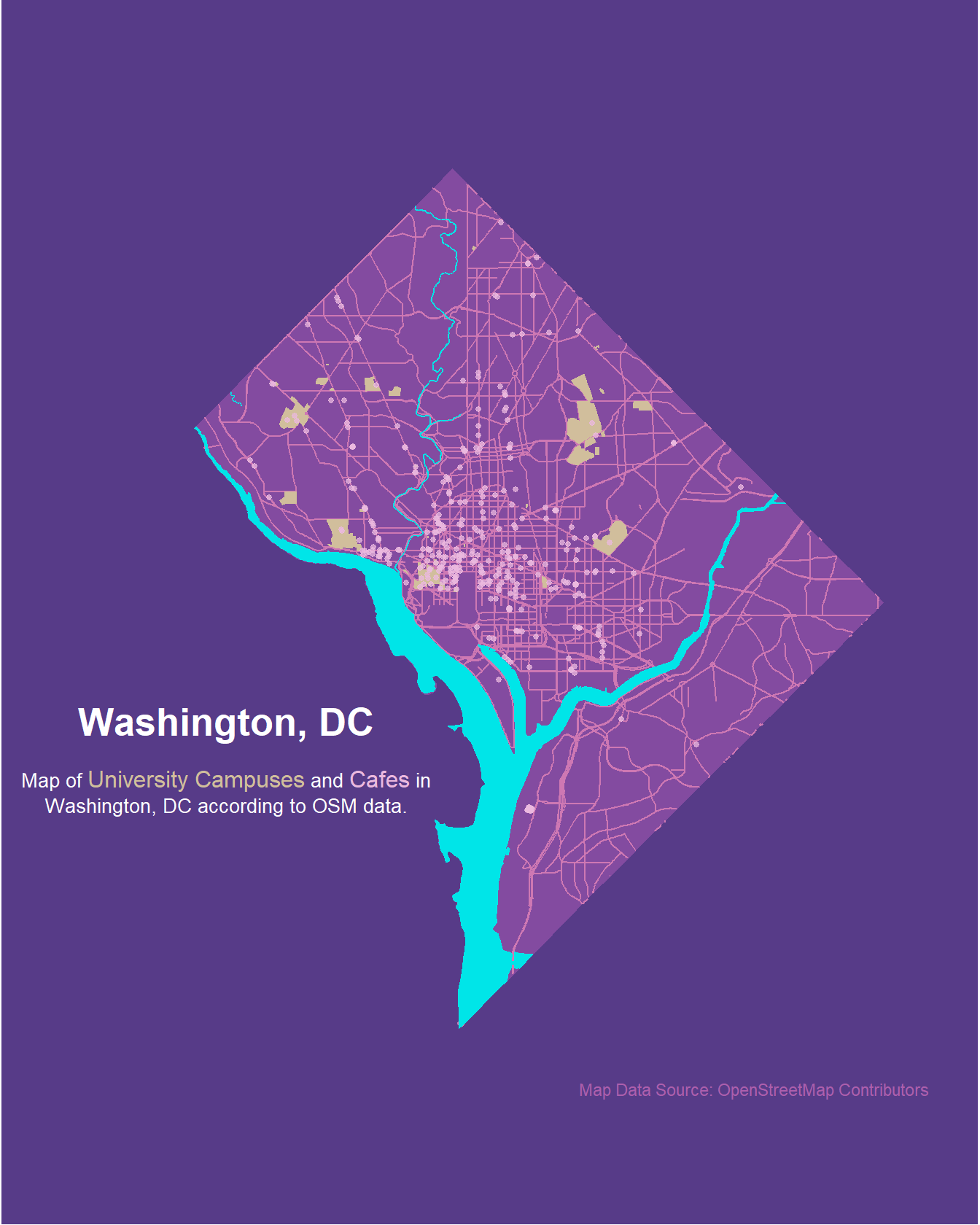
We’ll rely on the {sf}, {osmdata}, and {tidyverse} libraries to create a map of Washington, DC that includes information on university campuses and cafes a.k.a. the most important places for students.
We’ll start by getting the border polygon of Washington, DC with the getbb() function from the {osmdata} library as an {sf} object. We then select the main polygon only.
# Get DC borders
dcosmborders <- getbb("washington dc", format_out = "sf_polygon")
dcosmborders <- dcosmborders[1,] # Only main polygon
Next, the code uses the opq() and add_osm_feature() functions from the {osmdata} library to get data on the city’s streets and filter it to only include “motorway”, “primary”, “secondary”, and “tertiary” roads. The resulting data is then stored in the variable “streets” and is intersected with the city’s borders to ensure that the data only includes information within the city. The same method is applied to extract data for bodies of water, universities and cafes. Note that water has both polygons and multipolygons that need to be extracted separately.
# Get big streets
streets <- getbb("washington dc") |>
  opq() |>
  add_osm_feature(key = "highway",
                  value = c("motorway", "primary",
                            "secondary", "tertiary")) |>
  osmdata_sf()
streets <- streets$osm_lines |>
  st_intersection(dcosmborders)

# Water polygons
water <- getbb("washington dc") |>
  opq() |>
  add_osm_feature("water", "river") |>
  osmdata_sf()
water_poly <- water$osm_polygons |>
  st_intersection(dcosmborders)
water_multipoly <- water$osm_multipolygons |>
  st_intersection(dcosmborders)

# University polygons
university <- getbb("washington dc") |>
  opq() |>
  add_osm_feature("amenity", "university") |>
  osmdata_sf()
university <- university$osm_polygons |>
  st_intersection(dcosmborders)

# Cafes points
cafe <- getbb("washington dc") |>
  opq() |>
  add_osm_feature("amenity", "cafe") |>
  osmdata_sf()
cafe <- cafe$osm_points |>
  st_intersection(dcosmborders)
Finally, we leverage {ggplot2} functions to create the map itself including various customization for the map’s appearance, such as colors, text, and themes. The color palette was manually selected using the Coolors generator.
# Setting the title code in HTML for ggtext::geom_richtext
title <- "<span style='font-family:Arial;font-size:20pt;'>**Washington, DC**</span><br><br>
<span style='font-size:10pt;'>Map of <span style='font-size:12pt; color:#D1BE9C'>University Campuses</span> and <span style='font-size:12pt; color:#EBB9DF'>Cafes</span> in<br> Washington, DC according to OSM data.</span>"

# Plot
ggplot() +
  geom_sf(data = dcosmborders,
          color = "#834ba0",
          fill = "#834ba0") +
  geom_sf(
    data = streets,
    inherit.aes = FALSE,
    color = "#ce78b3",
    size = .4
  ) +
  geom_sf(
    data = water_poly,
    inherit.aes = FALSE,
    color = "#00E5E8",
    fill = "#00E5E8"
  ) +
  geom_sf(
    data = water_multipoly,
    inherit.aes = FALSE,
    color = "#00E5E8",
    fill = "#00E5E8"
  ) +
  geom_sf(
    data = university,
    inherit.aes = F,
    fill = "#D1BE9C",
    color = "#D1BE9C"
  ) +
  geom_sf(
    data = cafe,
    fill = "#EBB9DF",
    color = "#EBB9DF",
    size = 1,
    alpha = 0.75
  ) +
  scale_y_continuous(limits = c(38.79163, 38.99597)) +
  scale_x_continuous(limits = c(-77.15979, -76.89937)) +
  ggtext::geom_richtext(
    aes(x = -77.11, y = 38.855, label = title),
    color = "white",
    label.color = NA,
    fill = NA
  ) +
  labs(caption = "Map Data Source: OpenStreetMap Contributors") +
  theme_void() +
  theme(
    text = element_text(color = "white"),
    plot.caption = element_text(color = "#ad5fad", hjust = 0.95),
    plot.background = element_rect(fill = "#573b88", color = NA),
    plot.margin = margin(t = 65, r = 10, b = 65, l = 10, unit = "pt")
  )
…and the less artsy applications:
Open Street Map is a treasure trove for GIS data and its access has been greatly facilitated by the {osmdata} package leveraging the Overpass API. Exploring the geometries you can query with the API is easy with the purpose built function of the {osmdata} package. Simply use availiable_features() and availiable_tags() to see all available features. In addition to geometries you can also often scrape location specific information such as the website of a business or artists having designed a particular fountain. Examples of what one can do with that data includes computing walking distances to amenities and creating more minimalistic art-maps.
Epilogue:
And finally, here is the full code on howw you can make beautiful artistic maps with the OSM data API interface and {ggplot2}’s mapping capabilities in about 100 lines of code.
library(sf)
library(osmdata)
library(tidyverse)

# Get DC borders
dcosmborders <- getbb("washington dc", format_out = "sf_polygon")
dcosmborders <- dcosmborders[1,] # Only main polygon

# Get big streets
streets <- getbb("washington dc") |>
  opq() |>
  add_osm_feature(key = "highway",
                  value = c("motorway", "primary",
                            "secondary", "tertiary")) |>
  osmdata_sf()
streets <- streets$osm_lines |>
  st_intersection(dcosmborders)

# Water polygons
water <- getbb("washington dc") |>
  opq() |>
  add_osm_feature("water", "river") |>
  osmdata_sf()
water_poly <- water$osm_polygons |>
  st_intersection(dcosmborders)
water_multipoly <- water$osm_multipolygons |>
  st_intersection(dcosmborders)

# University polygons
university <- getbb("washington dc") |>
  opq() |>
  add_osm_feature("amenity", "university") |>
  osmdata_sf()
university <- university$osm_polygons |>
  st_intersection(dcosmborders)

# Cafes
cafe <- getbb("washington dc") |>
  opq() |>
  add_osm_feature("amenity", "cafe") |>
  osmdata_sf()
cafe <- cafe$osm_points |>
  st_intersection(dcosmborders)

title <- "<span style='font-family:galada;font-size:24pt;'>**Washington, DC**</span><br><br>
<span style='font-size:11pt;'>Map of <span style='font-size:13pt; color:#D1BE9C'>University Campuses</span> and <span style='font-size:13pt; color:#EBB9DF'>Cafes</span> in<br> Washington, DC according to OSM data.</span>"

ggplot() +
  geom_sf(data = dcosmborders,
          color = "#834ba0",
          fill = "#834ba0") +
  geom_sf(
    data = streets,
    inherit.aes = FALSE,
    color = "#ce78b3",
    size = .4
  ) +
  geom_sf(
    data = water_poly,
    inherit.aes = FALSE,
    color = "#00E5E8",
    fill = "#00E5E8"
  ) +
  geom_sf(
    data = water_multipoly,
    inherit.aes = FALSE,
    color = "#00E5E8",
    fill = "#00E5E8"
  ) +
  geom_sf(
    data = university,
    inherit.aes = F,
    fill = "#D1BE9C",
    color = "#D1BE9C"
  ) +
  geom_sf(
    data = cafe,
    fill = "#EBB9DF",
    color = "#EBB9DF",
    size = 1,
    alpha = 0.75
  ) +
  scale_y_continuous(limits = c(38.79163, 38.99597)) +
  scale_x_continuous(limits = c(-77.11979, -76.90937)) +
  ggtext::geom_richtext(
    aes(x = -77.09, y = 38.855, label = title),
    color = "white",
    label.color = NA,
    fill = NA
  ) +
  labs(caption = "Map Data Source: OpenStreetMap Contributors") +
  theme_void() +
  theme(
    text = element_text(color = "white"),
    plot.caption = element_text(color = "#ad5fad", hjust = 0.95),
    plot.background = element_rect(fill = "#573b88", color = NA),
    plot.margin = margin(
      t = 10,
      b = 10,
      l = 10,
      r = 10
    )
)Reuse
Citation
For attribution, please cite this work as:
Bieri, Bernhard. 2023. “Mapmaking with R and
OpenStreetMaps.” January 28, 2023. https://bernhardbieri.ch/blog/2023-01-28-mapmaking-with-r-and-openstreetmaps/.