Literate Programming in Stata

TLDR: Literate programming with Stata just became easier thanks to the recent release of Quarto and the continuingly increasing integration of Stata and Python. One can now render a .qmd Quarto file or a Jupyter notebook containing Stata chunks and create publishing grade outputs such as presentations, dashboards and reports at the click of a button! The prerequisites of this workflow are Stata 17, Quarto, Python, as well as a few standard Python libraries. Click here to jump to the detailed instructions and skip the intro.

What Literate Programming Is and Why You Should Care

Literate programming is a concept pioneered by Donald Knuth, a Turing Award recipient known for creating TeX. The main idea behind the early form of literate programming was to upend the traditional programming practices of the time by systematically including human readable text accompanying and explaining the logic and the purpose of a program. As he describes in “Literate Programming”, Knuth considers the programmer as an “essayist” who should strive to communicate the purpose of a program in order to create better code. While initially centered in the domain of computer science, it more recently resurged in the interdisciplinary world of “data science”.

The Resurgence of Literate Programming in the 2010’s

With the advent of data science in the past 20 years with its interdisciplinary nature, the need for human readable text accompanying code grew. This is due to the fact that the interpretation of the results of a computation lies at the center of every data science project. It is thus extremely important to include either comments in a code or leverage modern literate programming tools to communicate the purpose of one’s code.

Modern examples of this practice include Jupyter Notebooks for Python and the combination of the {knitr} package and the RMarkdown format for R. These tools allow data scientists to interweave computational output with the theoretical explanations necessary to interpret it. Thereby, they accelerate the production of scientific products such as papers, reports, dashboards, etc. However, Stata, one of the most widely used piece of statistical software still lags behind in this regard and does not provide its users with a native option to leverage literal programming workflows. Existing solutions include {markdoc} a Stata package that is akin to {knitr} in R and supports exports to PDF, HTML, Word, Markdown and other common formats. Recently, however, the Quarto revolution occurred within the R/Python community and paradoxically also changed the game for literate Stata workflows thanks to the latter’s integration with Python.

The Stata-Python-Quarto Workflow for Literate Programming

Quarto’s release earlier this summer added the missing link to the implementation of the Stata literate programming workflow described below. Quarto is essentially a language agnostic tool that enables data scientists to generate PDFs, Word Documents, dashboards and other outputs from code at the click of a button in R, Python, ObservableJS, etc. While Quarto does not work with Stata out of the box, the tighter integration of Python and Stata with the release of Stata 17 and the PyStata package enables a literate programming workflow!

In what follows, we will look at two options to use Quarto to generate similar static HTML reports based on this example script introducing Stata17’s new companion PyStata package. We will first look at how to handle classic Jupyter notebooks before moving on to rendering a native .qmd files. Both workflows are almost identical, hence if you’re used to Jupyter notebooks, simply stick to the first one. The second one may be more familiar for those migrating from R as the .qmd file structure is almost identical to the .Rmarkdown file structure.

Want to see the final product before we start? Check out the Jupyter notebook example and the native Quarto example.

A Few Prerequisites

Make sure that the following prerequisites are met before reading on. They are the same for rendering both Jupyter notebooks and .qmd files.

• Python
• VSCode (I found that it works best for this workflow due to the Quarto extension)
• Stata 17
• Quarto
• The Quarto extension for VSCode
• A few Python libraries and their dependencies:
  • Jupyter to run Jupyter Notebooks
  • Stata_setup to initialize the PyStata package which is located in the install folder of Stata 17

Additionally to run the example code, install the following packages and their dependencies:

• matplotlib

# Create new project env:
conda create --name StataPythonQuarto
# Activate it:
conda activate StataPythonQuarto
# To run the Jupyter Notebook:
pip install -U jupyter
# Stata bridge itself:
pip install -U stata_setup
# For matplotlib graph:
pip install -U matplotlib

Setting up your Project

Head to VSCode, select your new environment, and open up a new Jupyter notebook or a .qmd file in your project folder. The steps below are exactly the same in both cases, simply insert the code in Jupyter chunks in the first case and in .qmd chunks in the latter case.

The first thing you have to do before starting your data analysis workflow is to set the YAML header containing the metadata of your data science project. If you’re opting for a Jupyter notebook, you’ll need to insert it in a raw chunk at the very beginning of your notebook (see the example notebook for more details). In the case you’re running with a .qmd setup, simply copy put it at the top of your file.

---
title: Running Stata within a Jupyter Notebook and Rendering to HTML with Quarto.
author: Bernhard Bieri
date: "09-02-2022"
theme: "cosmo"
format: html
---

The next step is to import the PyStata package located in the install folder of your Stata distribution with the stata_setup.config() function. Simply run the following code chunk after inserting the YAML. Note that you need to specify the Stata version you have installed on your system. \(\in \{\text{be}\ ;\text{se}\ ;\text{mp}\}\).

# Setup Stata from within Python
import stata_setup
stata_setup.config("C:/Program Files/Stata17", "be")

After this you are good to go!

Running the Analysis

You can now import your data with your standard Python commands, clean them within Python before running your analysis and produce tables or graphical outputs with your favorite Stata commands.

See the following Jupyter notebook example and .qmd example for a complete workflow & output into HTML!

Previewing and Rendering your Project

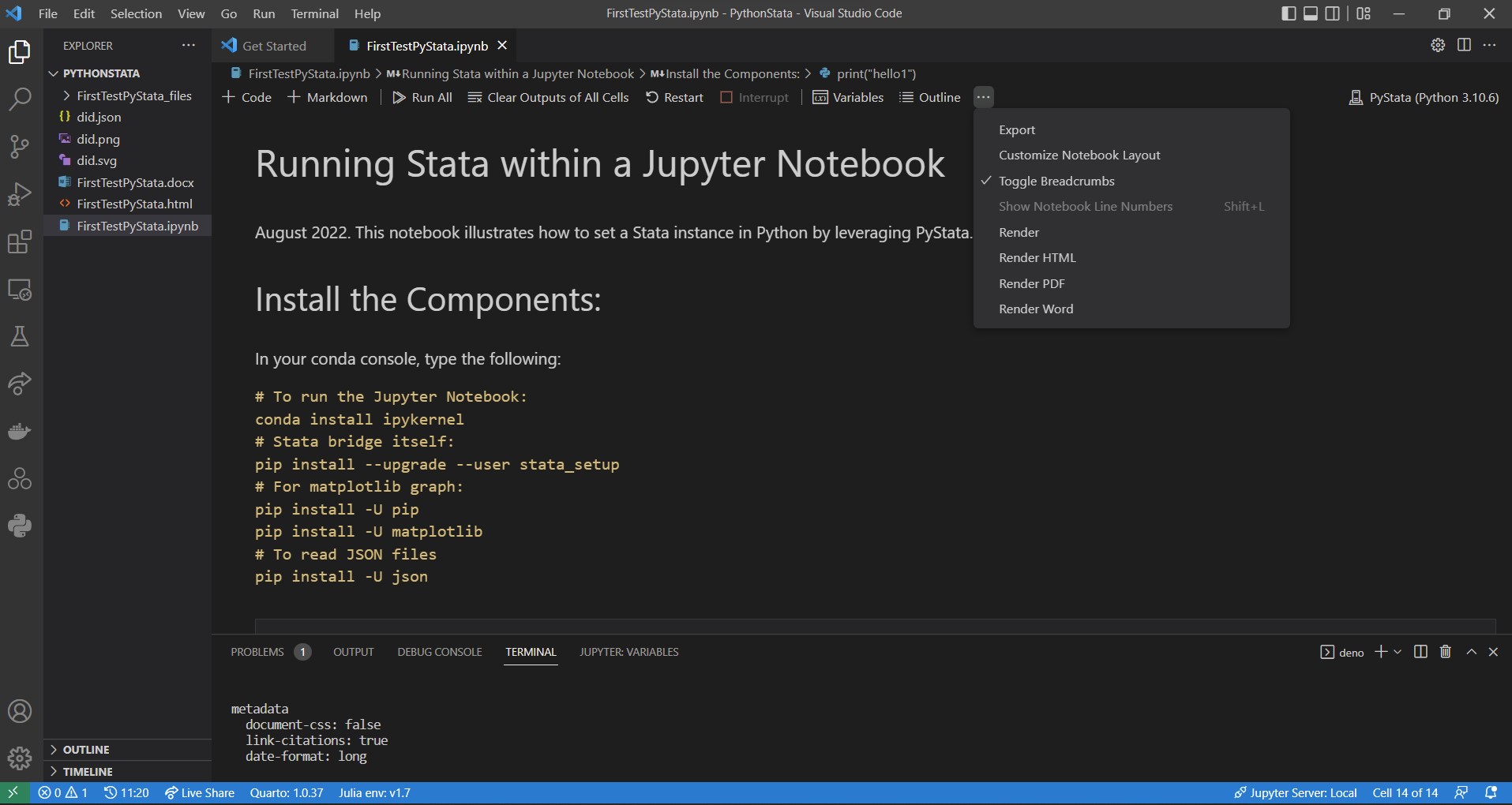
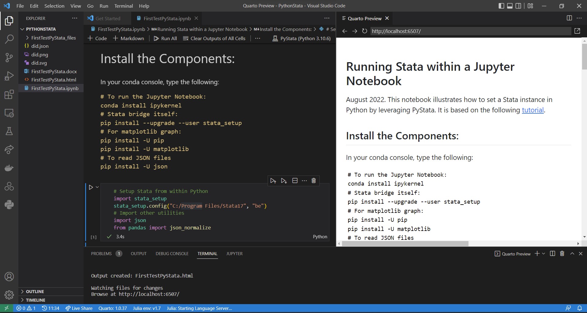
Rendering your report is a one click/one line thing! If you have VSCode and the Quarto extension installed, simply hit render in the menu bar as indicated on the screenshots below. This will execute all the code chunks in the background and weave together tables, graphs, and text. It will then open up a preview in a dedicated tab and save your final output in your root folder.

Bonus Tip: You can hit the CTRL/CMD + Shift + K key-binding to render your report even faster. It works for both Jupyter notebooks and .qmd files.

rendercommands

livepreview

Further Readings

Here are some useful websites to go further with your workflow.

• The awesome Quarto Documentation
• A great Appsilon Blog on Quarto
• What’s new in Stata 17